Deep learning for gesture recognition with a very small training set
I've finished my experiments with autoencoding (convolutional predictive sparse decomposition), and am happy to say that it works reaosnably well (at least as far as my tests went). I implemented a sophisticated autoencoding method in Python and Theano to learn features to supply an SVM classifier to distinguish 12 different hand poses with an 81% accuracy on a small balanced training set. All features were learned unsupervised.
The training set for the classifier consisted of 426 images (about 35 images per hand pose) and 53 test images. The autoencoder contained two layers and was first trained on all 479 64 x 64 pixel greyscale hand pose images.
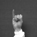
Example "V" pose with simple background used in learning.
Example "V" pose with complex background not used in learning.
The hand-pose images for training and testing did not include complex background cases. The point of the test was to demonstrate that the end-to-end system works on some level and most importantly to analyze the output of the unsupervised autoencoders. The complex background cases were harder.
The final implementation I completed is the "convolutional predictive sparse decomposition" or CPSD (
[1],
[2]), which also required writing an implementation of
FISTA in Python. As an aside, FISTA is a very cool optimization algorithm for finding the minimum of partially non-smooth convex functions (e.g. L1-regularized quadratic loss functions). FISTA has many applications including image enhancement (denoising, deblurring, superreslution), matrix completion (collaborative filtering), quantitative finance, and others. Everything I did was written from the ground-up in Python (
Theano was used for its symbolic differentiation capabilities, which are outstanding for this purpose).
As you can see, there are many extensions, but CPSD is quite a powerful algorithm even without the various extensions. Research papers advancing this technique are still being published as of 2015 (it was introduced around 2008/2010) and the citation network is really not that big (there aren't that many "experts" in this area). The concepts are not that difficult to understand, but implementing and tuning the architectures are both time-consuming and tricky undertakings.
Beyond 2D image classification, other applications of this approach include learning
3D convolutional filters in an unsupervised manner (width x height x time), which could lead to higher accuracy for static recognition as well as dynamic time-sequence recognition. Other types of data such as audio and time series data could benefit from this approach as well.
There are many things that could be tried to improve the results here including learning more filters and increasing filter size, adding more layers (avoiding dramatic downsampling steps), and adding a post-processing step that, for example, would learn to classify a final image from the output of some number of successive frames (e.g. temporal ensemble learning) or learning multiple classifiers and training a final ensemble classifier.
What does CPSD do? It finds "sparse," "overcomplete" basis elements for a distribution (a signal). The basis and distribution are inferred from a set of training examples. The result is a set of encoding filters and reconstruction bases. For example, let's say you find 8 encoding filters from a set of training examples. From these, you can take an input image and produce 8 filtered "images" such that each filtered version emphasizes some particular aspect of the original image. These filtered images are useful for classification purposes as they may highlight features characteristic of certain objects or regions of interest. This filtering is what a convolutional neural network does in feed-forward mode (e.g. post-training) repeatedly using several layers.

The above image shows the 8 encoding filters learned in the hand-pose recognition experiment described initially. This is an enlarged image of the eight 7 pixel x 7 pixel kernels. They were randomly initialized, but through the unsupervised learning process they became very functional oriented edge-detectors (Gabor-like filters). The filters are randomly initialized and from there, the learning process seeks to find a local optimal filter.
While the optimization does jointly consider all filters in the reconstruction, there are no guarantees that filters will cover some particular spectrum of variance of the input signal. For example, the filters are not guaranteed to be mutually orthogonal as is the case with the basis in principal component analysis. Larger filters presumably have more randomness with which to find that local optimum and more flexibility in describing complex shapes found in the input. There is also no guarantee that the entire filter area will be used, as can be seen from above. More filters provide a higher likelihood that the filters cover a greater spectrum of variance of the input.
What CPSD does is learn the filters for each layer of a feed-forward convolutional neural network without supervised backpropagation. Supervised backpropagation in a deep convolutional neural network is problematic because the error at the top level must be propagated back down each level. This results in a "vanishing gradient" problem wherein by the the time the error gets down to the bottom level, the adjustment that is made to the network is very small. So it takes a long time and a lot of training to adjust the parameters of all layers of the network enough to achieve good results. This is why "pretraining" is a popular research area.
There are (at least) two major pretraining techniques: stacked sparse autoencoders (e.g. LeCun) and deep belief networks (e.g. Hinton). Interestingly, a lot of research shows that completely random filters at the non-top layers of a deep convolutional neural network performs pretty well for "some" datasets (especially those with small numbers of training examples). Another technique is to use a large general-purpose trained network as a base and use a smaller set of training examples to refine the general-purpose trained network for a specific application. A large dataset and deep convolutional network can take weeks to train even with very advanced algorithms and hardware. By contrast, the layer-by-layer unsupervised pretraining techniques learn very fast as the gradient of the loss function of a layer is directly applied to the parameters of that layer and not propagated down.
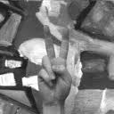
This image shows the highpass filtered "V" pose image being run through the 8 encoder filters. Each filter highlights a particular characteristic of the input.
In order to infer the parameters of these CPSD layers, the small dataset is repeatedly run through in an batch online stochastic gradient process. In this experiment, a few variations were applied to the images (horizontal reflection and small (5%) scale increments and decrements. Each epoch consisted of about 2,800 images (formed from the initial set of 479 hand-pose images). The filters took shape within about 4 epochs but a total of 10 epochs were run for both layers. With a batch size of 5, less than 6,000 gradient updates were required for each of the two layers to learn these filters. With batched online stochastic gradient, the gradient updates of each image in the batch could be computed in parallel as well (though this was not done for this). It was very important to carefully set the learning rate to achieve this fast learning but also avoid divergence.
For the non-linear activation function, I implemented a modification to the rectified linear unit (ReLU) called the "parametric rectified linear unit" or PReLU. I initially used the hyperbolic tangent but substituted the PReLU and found it learned the filters faster (though I can't say it gave better overall classification results). The important thing in these learning algorithms is finding a gradient that adjusts the parameters to a local minimum. With the hyperbolic tangent, there is a small range in which the gradient is non-zero. Outside of that range, the gradient is zero and the bias must adjust to move the filter back into regime where it can be updated. One of the problems with this is that if the learning rate for the bias is too fast, it will overshoot that small range and cause the loss to diverge. However making the bias updates smaller results in much longer training times. The rectified linear unit has a continuous gradient over a large range (all positive values). Unless the filters are initialized poorly, chances are good that the ReLU will allow the filters to converge quickly. The parametric rectified linear unit includes a parameter that provides some non-zero gradient for negative inputs. This is helpful to get the input "unstuck" if it becomes negative. The PReLU is actually a leaky ReLU with a learned leak-rate. No bias is needed for the PReLU (though I did include a gain parameter to help compensate for scale differences in the input).
A final note is the preprocessing of the input that is required. There were two important steps. The first is mean-centering and division by standard deviation. This helps to bring the inputs within a common scaled range. Pixel values were first converted to a range between 0 (black) and 1 (white). After this preprocessing, a highpass filter was applied consisting of the subtraction of a simple gaussian filter as well as another divisive normalization step. These steps converted input with a great deal of illumination, texture, and other variation into an edge-based representation. Learning in this space was much faster and yielded much better classification results.
CPSD is different from autoencoding in two ways. First, it is sparse and overcomplete. Non-sparse autoencoding results in a compressed (undercomplete) intermediate representation of the distribution being modeled. Going back to the example above, for autoencoding purposes in a non-sparse setting, the best filter to learn in an overcomplete setting (where, for example, 8 filters were learned for one input image) would be identity filters (e.g. kernels with 1 in their centers), which just pass on the input without modifying it. The sparse constraint forces the optimization to learn "interesting" non-identity filters. As it turns out, the filters learned at low-levels for highpass filtered natural images tend to look like Gabor filters (oriented edge detectors). This is what is claimed in research papers and this is what my implementation found as well. Check.
The second way that CPSD is different from autoencoding (and other sparse autoencoding methods) is that it operates on the entire image at once rather than on independent patches of the image. The patch-based approach tends to learn more redundant filters. The whole-image approach also has a better ability to discern more "interesting" shift-invariant features. This comes at a price, however, as the optimization loss function involve a convolution rather than the matrix-vector product in the patch-based approach. This requires a more complex optimization method than simple gradient descent, which is where FISTA comes in. FISTA attempts to find the minimum of a complicated function, which in this case is the reconstruction loss of the autoencoder with the sparsity penalty that is needed in overcomplete systems.
Images in their "raw" space (e.g. a 64x64 grayscale image contains 4,096 raw pixel-value dimensions) are difficult to classify. The hope is that by extracting features and projecting the raw pixel values into the more useful feature space that classification tasks will be easier. Convolutional neural networks repeatedly filter images (using the types of filters shown above) and pool the resulting filters. Usually the pooling includes a downsampling step. The architecture I constructed had two of these convolutional+pooling layers and the final dimensionality was about 1/4 of the original raw dimensionality.
This shows the same filtered images as above from the output of the first convolutional filters but downsampled through a 2x max-pooling operation.
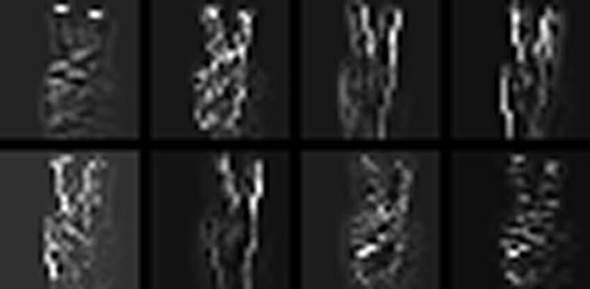
These are the 64 7x7 encoding filters learned in the second layer. Several of the filters still exhibit Gabor-like qualities but others include more object specific patterns and gratings.
This is the output of the second layer filters applied to the output of the first layer filters. A mapping and combination process is performed such that for each of these outputs (32 in total), two of the first layer outputs are convolved with two learned filters and then combined. This is why there are 64 filters shown above but only 32 output images. This is a common technique for increasing the coverage with respect to the variance of the input. In these filtered images, you can see different aspects are highlighted. Each of these images is now only 17 pixels by 17 pixels (2x downsampling from first layer and the various edge effects from convolution and local contrast normalization (highpass filtering).
Here is the same filtered output with another 2x downsampling.
And here is the filtered output with 4x downsampling.
In keeping with the principles of the
"spatial pyramid pooling" technique, the final output contains the 1x downsampling (i.e. no downsampling), the 2x downsampling, and the 4x downsampling outputs concatenated together as the final feature set. Despite the obscurity of the final 4x downsampling, these are critical features for the classification. This also demonstrates how pooling and downsampling helps to achieve shift-invariance. With max-pooling over the entire image (or large subareas of the image), the feature set becomes a "bag-of-words." For deep networks with lots of filters, this bag-of-words approach can be a very powerful way to achieve both shift and scale invariance.
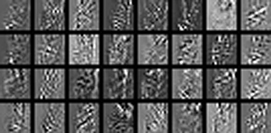
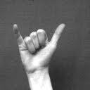
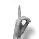
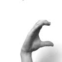
Here is another sample of the some of the other hand-pose classes: